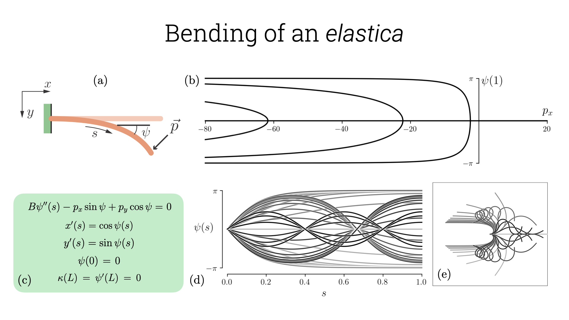
Before we start the tutorial, it might be useful to note that auto-07p codes for all the examples are available in this link. The first problem we will solve in this tutorial is the deformation of an inextensible slender filament known as the elastica. We solve this in 2-dimensions where the structure can be represented only using curvature information along the filament (captured up to global translations and rotations). The concept of an elastica is very old and dates back to the times of Bernoulli and Euler (read more about it here). We consider an elastica hinged at one end while the other end experiences a point force \vec{p}= (p_x, p_y). This problem is described in detail in Prof. Audoly’s lecture notes. The elastic energy under an externally applied point force is \begin{aligned}
\mathcal{E}=& \ \underbrace{\frac{1}{2} \int_0^L B \kappa^2(s) \ \text{d}s}_{\text{Bending energy}} - \underbrace{\int_0^L (p_x \cos \psi + p_y \sin \psi) \ \text{d}s}_{\text{Potential energy}}.\end{aligned} Here s is the arc-length and the first term in the above equation is the bending energy term while the next is the work done/stored potential energy due to the applied force. The work done is nothing but -\vec{p}.\vec{r}(L) where \vec{r}(L) is the end point. The equilibrium equation by extremising this energy or equivalently the Euler-Lagrange equation is \begin{aligned}
B \psi''(s) - p_x \sin \psi + p_y \cos \psi =& \ 0.\end{aligned} Since we have fixed end on one side, this translates to \psi(0) = 0 and a torque free boundary at the other side implies \kappa(L) = \psi'(L) = 0. This equation can be non-dimensionalized using L as the length-scale and (B/L) as the energy scale. After non-dimensionalization we get \psi''(s) - p_x \sin \psi + p_y \cos \psi = 0. The rescaled forces are \tilde{p}_i = p_i/(BL^2),\ i=x, y (we have dropped the tildes for simplicity).
| Constants | Description | Values for elastica |
|---|---|---|
ICP |
Continuation parameters | p_x/p_y |
NPAR |
Number of parameters | 4 |
IPS |
Type of problem | 4 for boundary value problems |
ISP |
Switch for bifurcation detection | 2 will identify all kinds |
NBC |
Number of boundary conditions | 4 |
ISW |
Mode for branch switching | 1 for normal, -1 for switching to different |
UZR |
User defined points for output | p_x/p_y |
UZSTOP |
User defined range for parameters | p_x \in [-80, 20] |
NPR |
Print & save every NPR steps | 20 |
In order to implement this equation in auto-07p we need to first convert it into a set of first order differential equations. We define u_1 = \psi(s), u_2 = \psi'(s) and this results in: \begin{aligned}
u_1' =& \ u_2,\\
u_2' =& \ p_x \sin u_1 + p_y \cos u_1.\end{aligned} We know from geometry that x'(s) = \cos \psi(s), y'(s) = \sin \psi(s), which can also be combined with the above equations to obtain a set of 4 equations. We supplement it with boundary conditions: u_1(0) = u_2(1) = x(0) = y(0) = 0.
*.f90/*.c, ScriptsFor each problem we are interested in solving in auto-07p , there are at least 3 files required: (i) The constant file (which has a filename as c.*) that inform auto-07p of the details of the problem and the numerical details required for the package to prepare the solver. (ii) FORTRAN/C file with the governing equations, boundary conditions, integral constraints and the variables that need to be probed from the solution in order to plot them later to understand the solution. (iii) The most important file in this set is the python script that runs auto-07p with the specified constants. The script will help us span the phase space and continue along different solution branches.
In Table. 1 we note some of the most important constants that we will use in this tutorial set. A very useful cheat-sheet is in the manual under the title “Quick reference” of chapter 10. The fortran code etica.f90 has the equations as a set of first order couple differential equations with (p_x, p_y) as the parameters to vary (we vary only one in this example). This file also has the initial solution for the specified parameters from which we need to continue in order to identify the bifurcations in the system. This is a subtle detail which needs to be kept in mind which is that you always need to know a solution to start continuation. In most cases, we are always able to find the trivial solution, like here \psi(s) = 0, x(s) = s, y(s) = 0 for p_x=p_y=0. An important thing to note is that the function PVLS has 3 parameters that probe the value of \psi(1), x(1), y(1).
etica = load('etica')
mu = run(etica)
mu = mu + run(mu,DS='-')
mu = mu + run(mu('BP1'),ISW=-1)
mu = mu + run(mu('BP1'),DS='-',ISW=-1)
mu = mu + run(mu('BP2'),ISW=-1)
mu = mu + run(mu('BP2'),DS='-',ISW=-1)
mu = mu + run(mu('BP3'),ISW=-1)
mu = mu + run(mu('BP3'),DS='-',ISW=-1)
# Relabel solutions
mu = relabel(mu)
# Save to b.mu, s.mu, and d.mu
save(mu,'mu')
# Plot bifurcation diagram
p = plot(mu)
p.config(bifurcation_y=['psi(1)'])
#clean the directory
clean()
wait()
The python script etica.auto runs the code and finds the bifurcation diagram for the specified set of parameters which we describe in detail now. We can run this code after installing auto-07p by simply typing auto etica.auto in the terminal. The first line in the script loads the files (c.etica, etica.f90) and the run command runs it for the specified constants. Since in the initial solution we start is for p_x =0 and from the constants file we see that p_x \in [-80, 20], running the code continues along the solution branch for p_x \in (0, 20]. We see that there are no bifurcations and we can now take a detour and change the direction of continuation by setting DS=’-’ which will continue now from p_x =20 \rightarrow -80. We find there are 3 bifurcation points that are displayed as BPi, which stands for Branch Point (other solution types are described in chapter 6 in the manual) and i=1,2,3 is the index of the branch point. We can now change the solution branch from the original branch, which is the straight configuration of the elastica, to the bent configuration using ISW=-1 and continue till p_x =-80. We then continue along the negative direction to identify the solution when elastica is bent the opposite direction. We then move to the next branch starting at BP2 and perform the same set of actions, similarly for BP3. All the results are then saved and can also be visualized using the plot interface. However we use the results saved in the s.mu to plot the solution. We briefly describe how this works and the implementation is provided in the plotElastica.ipynb.
When we save the results, auto-07p generates 3 files b.mu, s.mu, d.mu corresponding to bifurcation diagram, solution and diagnostics. The bifurcation diagram has information very similar to what is displayed in the terminal when we run the program but with finer resolution depending on the specified parameters. The solution file on the other hand get saved every textttNPR steps as specified in the constant file. Further the solution file is a single file with all the solutions and thus has a specific format in which it is saved. The initial lines in the file have the parameter values at which the solution is saved followed by the solution itself. We process the bifurcation diagram and the solution using python package pandas which makes it easy to segregate and plot the data.
I am sharing here the format of the output file taken from this link, which has valuable information on how to process the files and will help make sense of the jupyter-notebook I have shared.