Föppl-von Karman equations in 2D captures the buckling of a sheet/strip/beam. The morphology of the sheet is captured using the deformation field along the in-plane direction is u(x) and the displacement along the out-of-plane direction is w(x). The governing equations for this deformation field is \begin{aligned} S (u_{xx} + w_{x} w_{xx}) + f =& \ 0, \\ -B w_{xxxx} + S [ w_{x} u_{xx} + \frac{1}{2} w_{xx} (2 u_{x} + 3 w_{x}^2 ) ] + p =& \ 0.\end{aligned} S is the stretching modulus, given by S = E \xi and B the bending modulus is E I where I is the second moment of inertial of the organism, where \xi is the thickness of the sheet, E the Young’s modulus, f and p are the external forces per unit length.
We can non-dimensionalize the force balance equations using the body-length of the organism L as the length-scale and E the Young’s modulus of the material as the stress-scale. Further we know that S \sim E\xi, B \sim E \xi^3 and using this we can then write the non-dimensional equations as \begin{aligned}
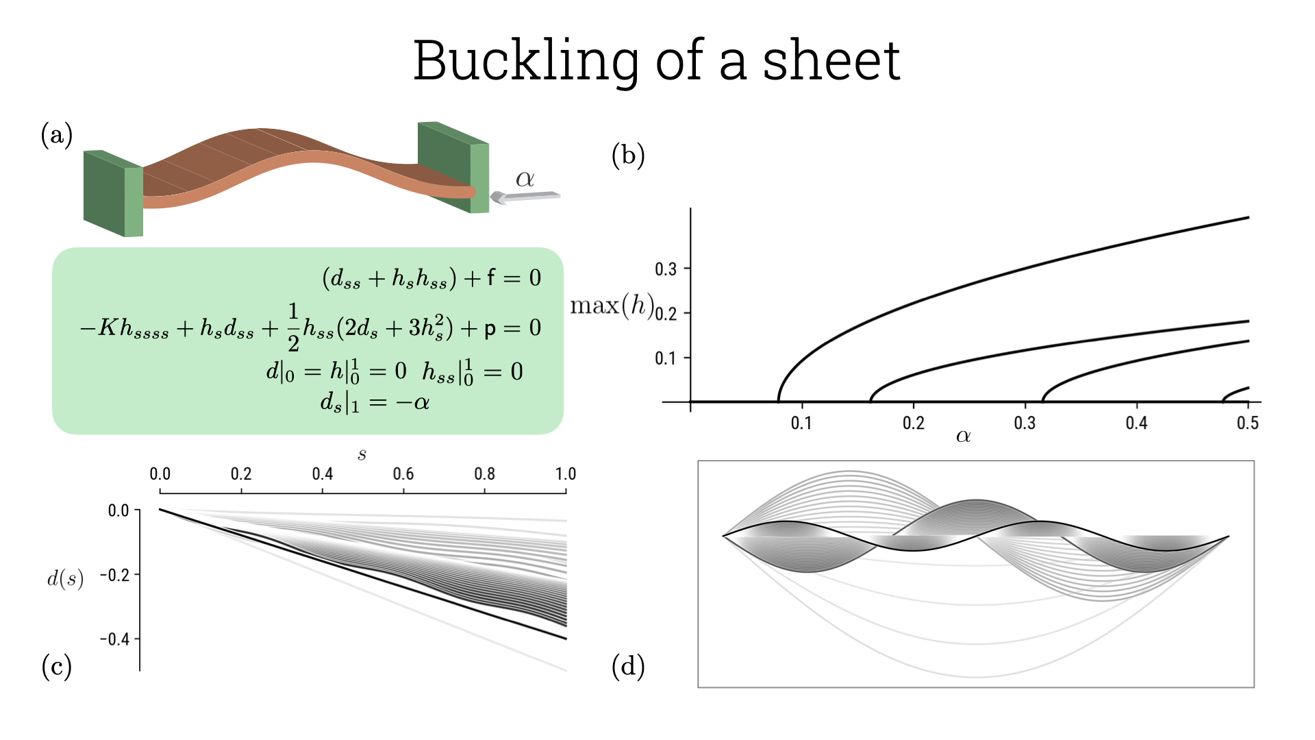
(d_{ss} + h_{s} h_{ss}) + \mathsf{f}=& \ 0, \\
- K h_{ssss} + h_{s} d_{ss} + \frac{1}{2} h_{ss} (2 d_{s} + 3 h_{s}^2) + \mathsf{p} =& \ 0,\end{aligned} where x= sL, u = dL, w = hL, K = (\xi/L)^2 is the geometric quantity highlighting slenderness, also known as the von Kármán number, \mathsf{f}= (fL/E\xi), \mathsf{p} = (p L/E\xi) are the non-dimensional forces. We can solve this system with the following boundary conditions: fixed ends, d|_0 = h|_0^1 = 0; zero applied moments, h_{ss}|_0^1 = 0; applied tangential strain, d_s|_1 = -\alpha. We can again perform a similar analysis to that of the elastica for a fixed value of K and changing the applied strain and is shown in the figure below. The code corresponding to these plots is in the 1parameter folder inside Tutorial2_FvK.
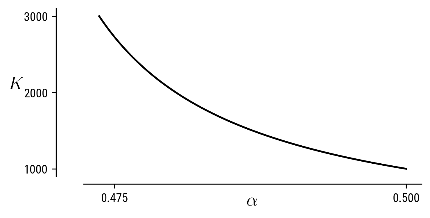
The leverage we have using the .auto script is that we can now steer the solution branch by varying different parameters in the equation. Once you have shifted from the unbuckled configuration to a bucked one using ISW=-1 (just as in the elastica case), we can change the continuation parameter to a different one, say K just by manipulating the .auto script. We can go further using auto-07p and continue the solution by varying both (K, \alpha) by using the variable ICP and setting limits using the UZSTOP command. For example we continue along two variables here by adding an integral constraint. This is because we need to satisfy the constraint NCONT = NBC+NINT-NDIM+1 where NCONT-number of continuation parameters, NINT-number of integral constraints, NDIM-number of dimensions. In the current problem we have NBC=6, NDIM=6 and thus we need an integral constraint to be able to perform continuation along the two-parameter phase space. After performing this, we get a isocontours in (K, \alpha)-plane representing morphologies of the sheet (a sample is shown in the figure below).