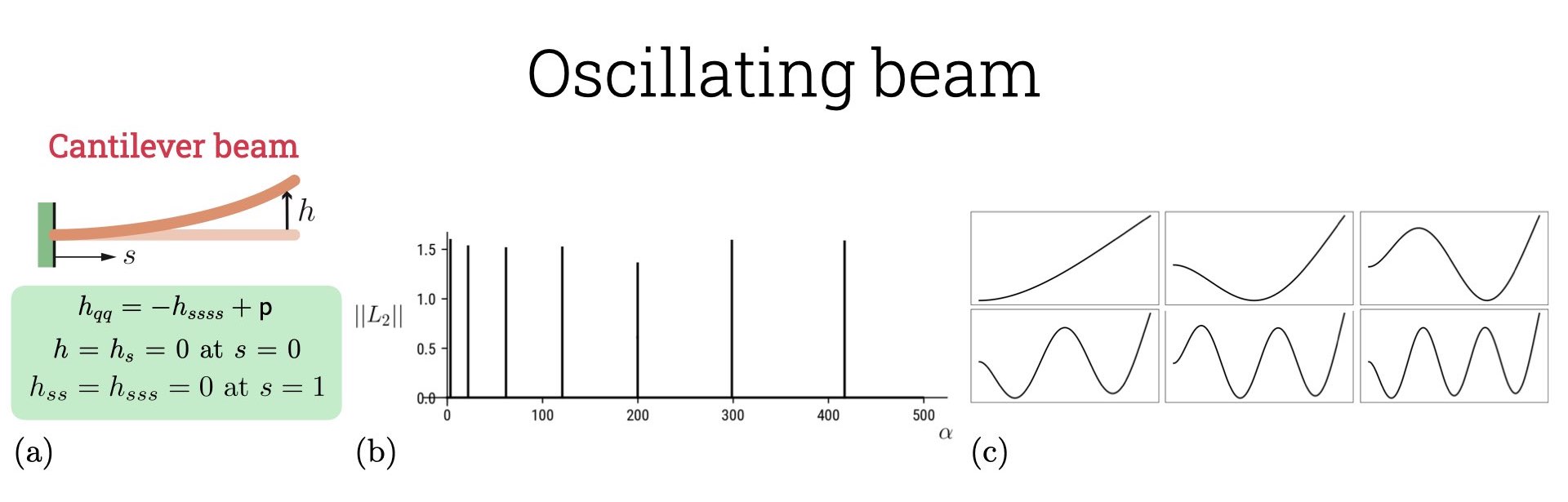
The small deflection theory capturing the morphology of an elastic beam is given by the Euler-Bernoulli equation which reads as \[\alpha w_{tt} = - B w_{xxxx} + p.\] Here \(w(x)\) is the vertical displacement along the beam’s length, \(\alpha\) is the mass per unit length, \(B = EI \sim E \xi^4\) is the bending modulus, \(E\) the Young’s modulus, \(I\) the second moment of area, \(\xi\) is the beam thickness and \(p\) is the body force per unit length. We can non-dimensionalize the equation with beam length \(L\) as the length scale, \(T \sim (\alpha L^4/B)^{1/2}\) as the time-scale and \(E\) as the stress-scale. Rewriting \(x = sL, t = qT, w = hL\), we can write the non-dimensional equation as \[h_{qq} = - h_{ssss} + \mathsf{p}.\] Here the non-dimensional body force \(\mathsf{p} = (pL^3/B)\). We are interested in solving this system for the boundary conditions: \((i)\) cantilever beam, \(h = h_s = 0\) at \(s = 0\), \(h_{ss} = h_{sss} = 0\) at \(s = 1\), with \({\mathsf{p}}=0\), \((ii)\) unsupported beam, \(h_{ss} = h_{sss} = 0\) at \(s = 0, 1\) with \({\mathsf{p}}=\beta \sin(2\pi s)\).
Though auto-07p is capable of solving discretized PDEs, we are interested in solving an eigenvalue problem which is coherent with our requirement to find oscillating solutions to the beam displacement. This can be done by substituting \(h(s, q) = \Re [ \hat{h}(s) \text{e}^{i \omega q} ]\) into the above equation, we then get \[\omega^2 \hat{h}= \hat{h}_{ssss} - \hat{\mathsf{p}}.\] For the cantilever beam we have the frequency of oscillation as the continuation parameter and this eigenvalue problem can be solved with the specified boundary condition in auto-07p. This is shown in the figure attached. The interesting aspect of the second problem of an unsupported beam is that the boundary conditions are all derivatives in \(h\) and thus do not provide a unique solution. One often needs to introduce pinning conditions to select form infinite translationally invariant solution. In auto-07p we do this by introducing a body forcing in the governing equation to get \[\omega^2 \hat{h}= \hat{h}_{ssss} - \hat{\mathsf{p}} + \lambda \hat{h}.\] and start the continuation with \(\lambda = 1\) from which point we continue towards \(\lambda = 0\). After we do this, we are free to continue along any direction as the initial solution is pinned and we have found one of the many solutions for \(\lambda = 0\). In the code attached Tutorial3_EB, we can have explored the solution for \(\omega = 1\) and continued the solution for different \(\beta\). This technique of continuing along one branch and then shifting to a different branch is called homotopy continuation. The boundary condition is not really physical here and the solution is not interesting either but I chose this condition to illustrate this technique which is super useful in a variety of scenarios.