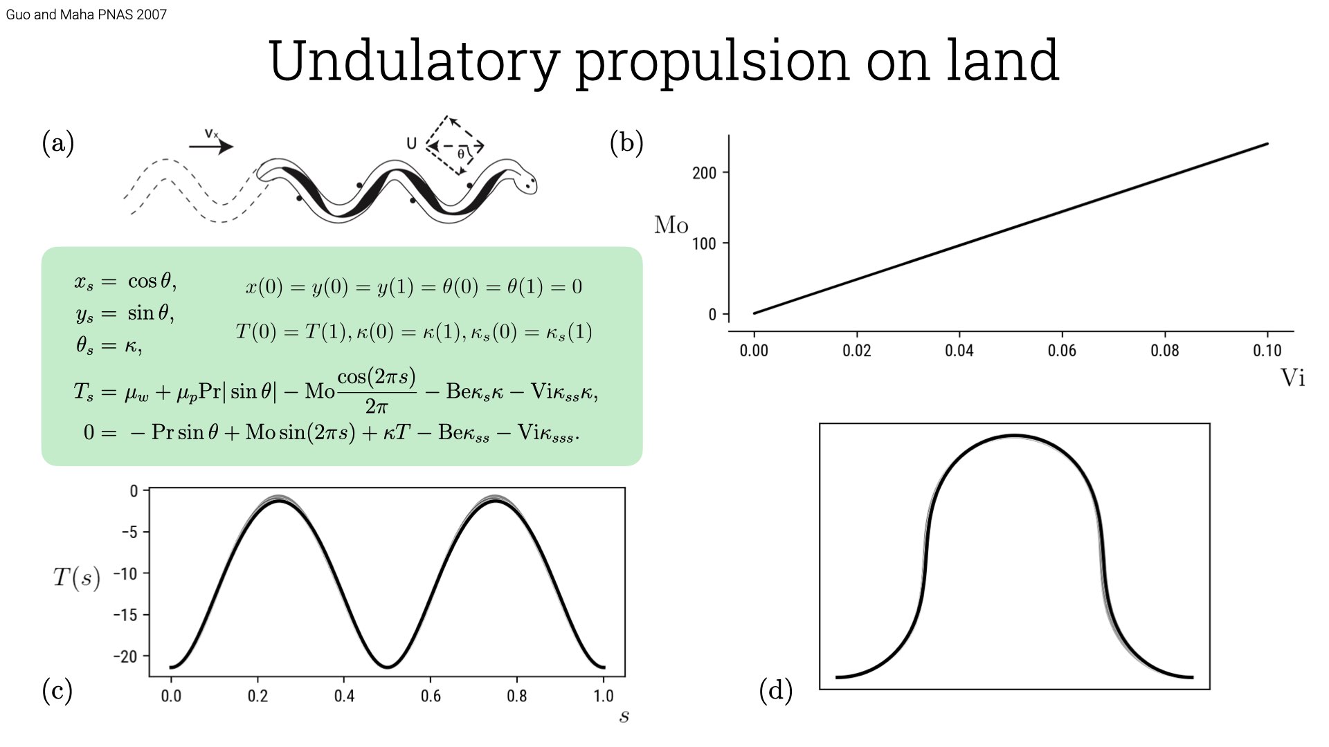
In this last tutorial, an attempt at coup de grace, we will be combining various techniques we have learnt in this tutorial and apply to the problem of locomotion on land by an active filament aka snake. Solving the problem in auto-07p is challenging as there are several parameters in the system. Further we need to impose periodic boundary conditions, which we have not yet seen in this series. The problem is solved by Guo and Maha, PNAS 2007 where they describe the shape of a snake based on the body centerline. Please refer to the article for a detailed derivation, the equations read \[\begin{aligned}
x_s =& \ \cos \theta, \\
y_s =& \ \sin \theta, \\
\theta_s =& \ \kappa, \\
T_s =& \ \mu_w + \mu_p \text{Pr} | \sin \theta| - \text{Mo} \frac{\cos (2\pi s)}{2\pi} - \text{Be} \kappa_s \kappa - \text{Vi} \kappa_{ss} \kappa, \\
0 =& \ - \text{Pr} \sin \theta + \text{Mo} \sin(2\pi s) + \kappa T - \text{Be} \kappa_{ss} - \text{Vi} \kappa_{sss}.\end{aligned}\] Here \(x, y\) are the position of the centerline, \(s\) is the arc-length, \(\theta\) is the orientation of the tangent along the body, \(\kappa\) is the curvature and \(T\) is the tension. There are 6 parameters in the system and they are Pr, Mo, Be, Vi, \(\mu_w, \mu_p\). The boundary conditions that supplement these equations are of two types, dirichlet and periodic. The dirichlet ones are: \(x(0) = y(0) = y(1) = \theta(0) = \theta(1) = 0\), while the periodic ones include: \(T(0)=T(1), \kappa(0) = \kappa(1), \kappa_s(0) = \kappa_s(1)\). As we have seen in our earlier tutorial, NCONT = NBC+NINT-NDIM+1. We have NDIM = 7 NBC=8, so we have two continuation parameters. We would like to find Mo vs Vi, just as in the paper.
In order to do that we split the task into two parts (problem is too hard to solve in one go). The first part is to enforce periodic boundary condition for most but not all the variables (this give confidence in the solution itself), continue from a numerically easily accessible solution to a point close to the actual region of interest. In the second part enforce the last periodic boundary condition that was not supplied earlier. In effect the first part ensure we are continuing along one branch by varying only one parameter and in the second we use homotopy continuation to asymptotically satisfy the last boundary condition. The itemize the steps taken and Snake.auto has the implementation of the method described here.
Initialize: \(x(s) = s, y(s) = \theta(s) = \kappa(s) = \kappa_s(s) = \kappa_{ss} = T(s) = 0\).
Choose starting parameters: Pr = 0.18, Mo = 0.0, Be = 0.4, Vi = 1.0, \(\mu_w\) = 0.0, \(\mu_p\) = 0.2. The starting parameters are close to the one in the Guo and Maha’s paper except for Mo, \(\mu_w\) and Vi. These parameter we shall continue to the exact parameters in the paper. I chose these parameters upon some experimentation to see to what extent auto-07p is stable when we start with a trivial guess for snake shape we have chosen.
Enforce boundary conditions: \(x(0) = y(0) = y(1) = \theta(0) = \theta(1) = 0\) and \(T(0)=T(1), \kappa(0) = \kappa(1)\). We have skipped \(\kappa_s(0) = \kappa_s(1)\), which we shall satisfy using homotopy continuation. As have NBC=7, we can continue only along one parameter. We shall add the additional boundary condition at the end and identify Mo vs Vi.
We pin the solution by the same technique we discussed earlier by defining a new parameter \(\lambda\) and set it to 1 initially which we will continue to 0 later. The equations them become: \[\begin{aligned} T_s =& \ \mu_w + \mu_p \text{Pr} | \sin \theta| - \text{Mo} \frac{\cos (2\pi s)}{2\pi} - \text{Be} \kappa_s \kappa - \text{Vi} \kappa_{ss} \kappa - \lambda T, \\ 0 =& \ - \text{Pr} \sin \theta + \text{Mo} \sin(2\pi s) + \kappa T - \text{Be} \kappa_{ss} - \text{Vi} \kappa_{sss} - \lambda \kappa.\end{aligned}\] This is done because the periodic boundary condition provides only translationally invariant solutions.
We start the continuation by varying Mo which has the body force and see that the shape of the snake change as we increase the amplitude.
We then continue from Mo = 100 by varying \(\lambda \rightarrow 0\).
We then vary \(\mu_w\), followed by varying Vi i.e. \(\mu_w = 0.1\), Vi = 0.03 to the actual parameters in the paper.
The most important step and really the crux of this tutorial is now to enforce the new boundary condition \(\kappa_s(0) = \kappa_s(1)\). This is done by having a new equations file (we call SnakeFull.f90) with the additional boundary condition added but with an additional parameter: \(\kappa_s(0) - \kappa_s(1) + \texttt{PAR(8)} = 0\). When \(\texttt{PAR(8)} \rightarrow 0\), we satisfy the boundary condition exactly. We need to also supply a new constants file with NPAR, NBC updated.
We can continue along Vi with Mo as the free parameter once we have satisfied all the boundary conditions and obtain the figure in the article which we show below.
