Bending of an elastica
Before we start the tutorial, note that auto-07p codes for all examples are
available at this link.
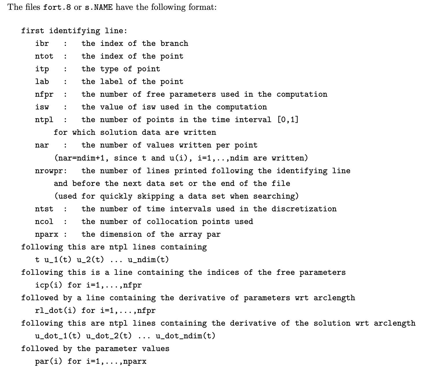
The first problem is the deformation of an inextensible slender filament known as the
elastica. We solve this in 2D where the structure can be represented using curvature
information along the filament. We consider an elastica hinged at one end while the other
experiences a point force \vec{p}= (p_x, p_y). The elastic
energy under an externally applied point force is
Here s is the arc-length. Extremising this energy gives the Euler–Lagrange equation
B \psi''(s) - p_x \sin \psi + p_y \cos \psi = 0.After non-dimensionalisation using L as the length-scale and (B/L) as the energy scale we get \psi''(s) - p_x \sin \psi + p_y \cos \psi = 0 with boundary conditions u_1(0) = u_2(1) = x(0) = y(0) = 0. Setting u_1 = \psi(s), u_2 = \psi'(s):
\begin{aligned} u_1' =& \ u_2,\\ u_2' =& \ p_x \sin u_1 + p_y \cos u_1. \end{aligned}Constants, *.f90/*.c, Scripts
For each problem in auto-07p there are at least 3 required files:
(i) the constant file (c.*),
(ii) a FORTRAN/C file with the governing equations and
boundary conditions, and (iii) a Python script
(.auto) that runs auto-07p and steers the continuation.
| Constant | Description | Value (elastica) |
|---|---|---|
ICP | Continuation parameters | p_x / p_y |
NPAR | Number of parameters | 4 |
IPS | Type of problem | 4 for BVPs |
ISP | Bifurcation detection | 2 — all kinds |
NBC | Number of boundary conditions | 4 |
ISW | Branch-switching mode | 1 normal, −1 switch |
UZSTOP | Parameter range | p_x \in [-80, 20] |
NPR | Save every NPR steps | 20 |
The Python script etica.auto runs and finds the bifurcation diagram:
# Load files c.etica and etica.f90
etica = load('etica')
mu = run(etica)
mu = mu + run(mu, DS='-')
mu = mu + run(mu('BP1'), ISW=-1)
mu = mu + run(mu('BP1'), DS='-', ISW=-1)
mu = mu + run(mu('BP2'), ISW=-1)
mu = mu + run(mu('BP2'), DS='-', ISW=-1)
mu = mu + run(mu('BP3'), ISW=-1)
mu = mu + run(mu('BP3'), DS='-', ISW=-1)
mu = relabel(mu)
save(mu, 'mu')
p = plot(mu)
p.config(bifurcation_y=['psi(1)'])
clean()
wait()
Running auto etica.auto continues from p_x = 0
in both directions. Three bifurcation points (BP1, BP2, BP3)
are found and branch-switched using ISW=-1, tracing bent elastica configurations.
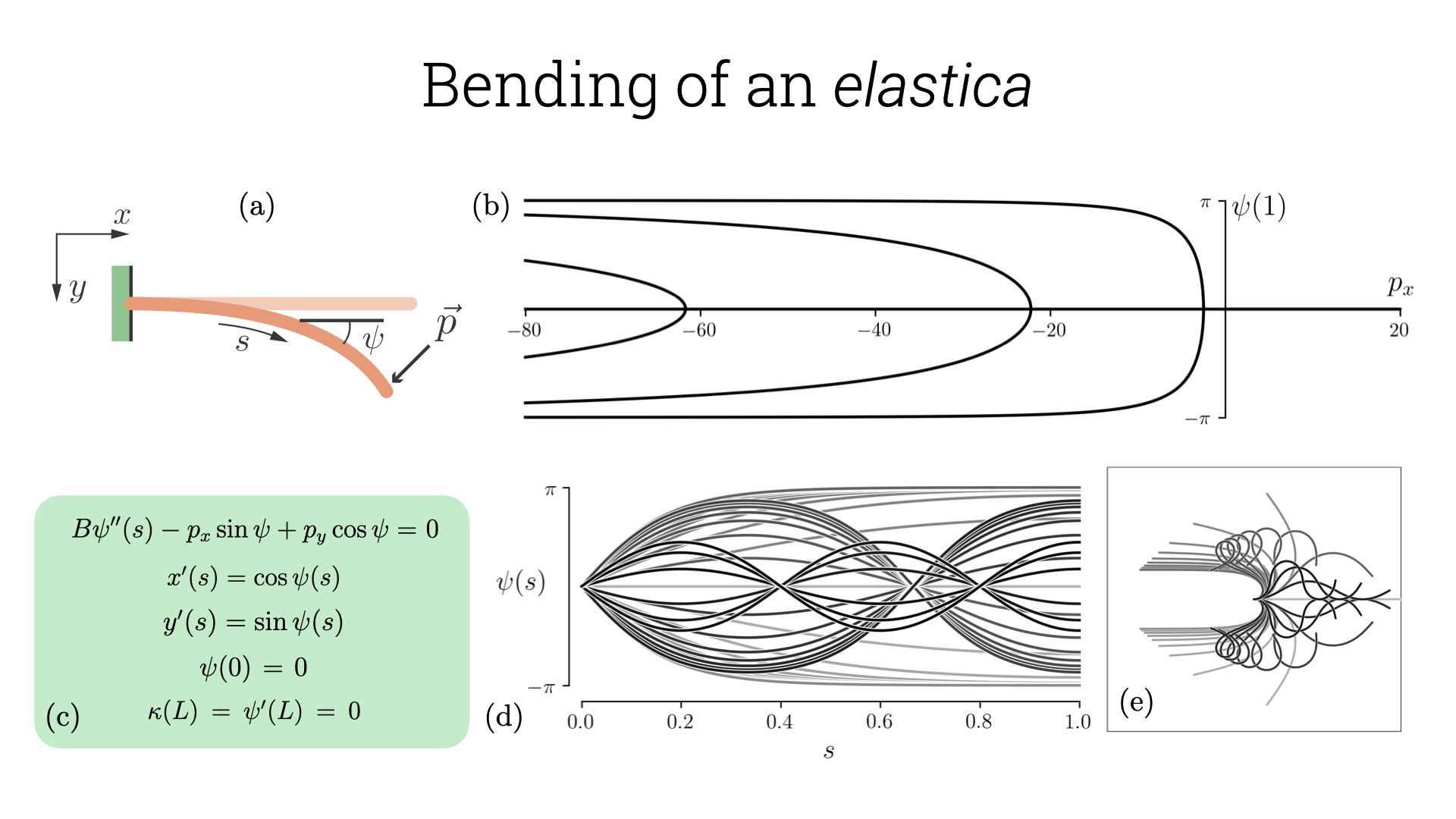
Results are saved as b.mu, s.mu, d.mu; solutions are post-processed via
pandas in
plotElastica.ipynb.
The format of the output file (from this reference) is shown below: